 A. We may also say that x "belongs to" A, or that x "is in" A.
 By Bruce Hoppe
| If your browser does not support mathematical symbols, you will not see this document correctly. If "⊆" looks like a box in quotes instead of a lazy U, or this math-symbol-test-page looks like a bunch of boxes, then you need to find a browser that supports mathematical symbols. In our experience, Firefox works and Internet Explorer does not. |
Introduction to Network Mathematics provides college students with basic graph theory to better understand the Internet. Many passages are edited from Wikipedia, a few are from PlanetMath, and others are original writing by Bruce Hoppe, who teaches CS-103: "Introduction to Internet Technologies and Web Programming" at Boston University. This is a work in progress, first created in the spring semester of 2007, and now being used in the fall semester 2008.
Copyright © 2007, 2008 by Bruce Hoppe. Permission is granted to copy, distribute and/or modify these documents under the terms of the GNU Free Documentation License, Version 1.2 or any later version published by the Free Software Foundation; with no Invariant Sections, with no Front-Cover Texts, and with no Back-Cover Texts. A copy of the license is included in the section entitled "GNU Free Documentation License". If you believe a portion of this site infringes on your or anyone's copyright, please send us a note.
A set is a collection of objects. These objects are called the elements or members of the set. Objects can be anything: numbers, people, other sets, etc. For instance, 4 is a member of the set of all even integers. Clearly, the set of even integers is infinitely large; there is no requirement that a set be finite.
If x is a member of A, then we write x A. We may also say that x "belongs to" A, or that x "is in" A.
If x is not a member of A, then we write x  A.
A.
Two sets A and B are defined to be equal when they have precisely the same elements, that is, if every element of A is an element of B and every element of B is an element of A. Thus a set is completely determined by its elements; the description is immaterial. For example, the set with elements 2, 3, and 5 is equal to the set of all prime numbers less than 6.
If the sets A and B are equal, then we write A = B.
We also allow for an empty set, a set without any members at all. We write the empty set as { }.
Explicit Set Notation: The simplest way to describe a set is to list its elements between curly braces, known as defining a set explicitly. Thus {1,2} denotes the set whose only elements are 1 and 2. Note the following points:
Warning: This notation can be informally abused by saying something like {dogs} to indicate the set of all dogs, but this example would be read by mathematicians as "the set containing the single element dogs".
The simplest possible example of explicit set notation is { }, which denotes the empty set.
Implicit Set Notation: We can also use the notation {x : P(x)} to denote the set containing all objects for which the condition P holds, known as defining a set implicitly. For example, {x : x is a real number} denotes the set of real numbers, {x : x has blonde hair} denotes the set of everything with blonde hair, and {x : x is a dog} denotes the set of all dogs.
Given two sets A and B we say that A is a subset of B if every element of A is also an element of B. Notice that in particular, B is a subset of itself; a subset of B that isn't equal to B is called a proper subset.
If A is a subset of B, then one can also say that B is a superset of A, that A is contained in B, or that B contains A. In symbols, A ⊆ B means that A is a subset of B, and B ⊇ A means that B is a superset of A. For clarity, we use "⊆" and "⊇" for subsets (which allow set equality) and we use "⊂" and "⊃" are reserved for proper subsets (which exclude equality).
For example, let A be the set of American citizens, B be the set of registered students at Boston University, and C be the set of registered students in CS-103. Then C is a proper subset of B and B contains C, which we can write as C ⊂ B andB ⊃ C. If we allow the possibility that every BU student might be registered for CS-103, then we would write C ⊆ B or B ⊇ C to allow for this unlikely situation. Note that not all sets are comparable in this way. For example, it is not the case either that A is a subset of B nor that B is a subset of A.
Given two sets A and B, the union of A and B is the set consisting of all objects which are elements of A or of B or of both. It is written as A ∪ B.
The intersection of A and B is the set of all objects which are both in A and in B. It is written as A ∩ B.
Finally, the relative complement of B relative to A, also known as the set theoretic difference of A and B, is the set of all objects that belong to A but not to B. It is written as A \ B. Symbolically, these are respectively
A) or (x B)} A) and (x B)} A) and not (x B) }Notice that B doesn't have to be a subset of A for A \ B to make sense.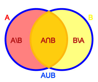
To illustrate these ideas, let A be the set of left-handed people, and let B be the set of people with blond hair. Then A ∩ B is the set of all left-handed blond-haired people, while A ∪ B is the set of all people who are left-handed or blond-haired or both. A \ B, on the other hand, is the set of all people that are left-handed but not blond-haired, while B \ A is the set of all people that have blond hair but aren't left-handed.
Venn diagrams are illustrations that show these relationships pictorally. The above example can be drawn as the Venn diagram at right:
Disjoint sets: Let E be the set of all human beings, and let F be the set of all living things over 1000 years old. What is E ∩ F in this case? No human being is over 1000 years old, so E ∩ F must be the empty set { }. When the intersection of any two sets is empty, we say those two sets are disjoint.
Intuitively, an ordered pair is simply a collection of two objects such that one can be distinguished as the first element and the other as the second element, and having the fundamental property that two ordered pairs are equal if and only if their first elements are equal and their second elements are equal.
We write an ordered pair using parentheses--not curly braces, which are used for sets. For example, the ordered pair (a,b) consists of first element a and second element b.
Two ordered pairs (a,b) and (c,d) are equal if and only if a = c and b = d.
In contrast, a set of two elements is an unordered pair which we write using curly braces and where there is no distinction between the first element and the second element. It follows thatA partition of a set X 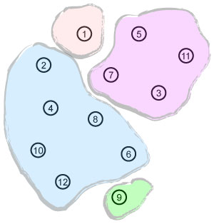 is a division of X into non-overlapping subsets such that every element of X is in exactly one of these subsets.
Equivalently, a set P of subsets of X, is a partition of X if
We also typically require that each subset of a partition be non-empty. For example:
 graph theory in order to study all kinds of networks. A graph is a set of objects connected by lines.
The objects in a graph are usually called nodes or vertices. The lines connecting the objects are usually called links or edges.
More formally, we define a graph G as an ordered pair G = (V,E) where
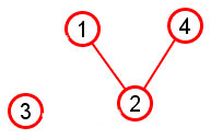
Example: The picture above represents the following graph:
 Unless explicitly stated otherwise, we disallow loops.
Undirected graph: The edges of a graph are assumed to be unordered pairs of vertices. Sometimes we say undirected graph to emphasize this point. In an undirected graph, we write edges using curly braces to denote unordered pairs. For example, an undirected edge {2,3} from vertex 2 to vertex 3 is the same thing as an undirected edge {3,2} from vertex 3 to vertex 2.
Directed graph: In a directed graph, the two directions are counted as being distinct directed edges. In an directed graph, we write edges using parentheses to denote ordered pairs. For example, edge (2,3) is directed from 2 to 3 , which is different than the directed edge (3,2) from 3 to 2. Directed graphs are drawn with arrowheads on the links, as shown below: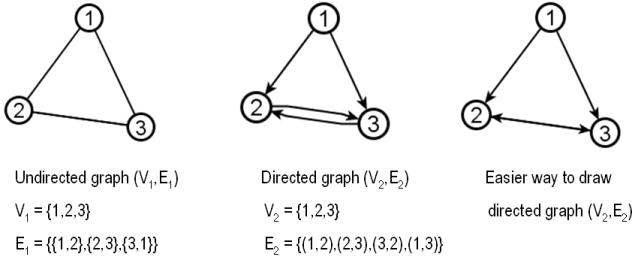
Two vertices are called adjacent if they share a common edge, in which case the common edge is said to join the two vertices. An edge and a vertex on that edge are called incident.
See the 6-node graph below right for examples of adjacent and incident:
The undirected graph at right has the following degrees:
| Vertex | Degree |
|---|---|
| 1 | 2 |
| 2 | 3 |
| 3 | 2 |
| 4 | 3 |
| 5 | 3 |
| 6 | 1 |
In a directed graph, we define degree exactly the same as above (and note that "adjacent" does not imply any direction or lack of direction). It is also important to define indegree and outdegree. Recall that any directed edge has two distinct ends: a head (the end with an arrowhead) and a tail. Each end is counted separately. The sum of head endpoints count toward the indegree of a vertex and the sum of tail endpoints count toward the outdegree of a vertex. The directed graph at right has the following degrees, indegrees, and outdegrees: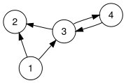
| Vertex | Degree | Indegree | Outdegree |
|---|---|---|---|
| 1 | 2 | 0 | 2 |
| 2 | 2 | 2 | 0 |
| 3 | 3 | 2 | 2 |
| 4 | 1 | 1 | 1 |
Pay particular attention to nodes 3 and 4 in the above table. If they seem confusing, try re-drawing the above graph using the "easier way to draw" illustrated previously.
The graph density of a graph G = (V,E) measures how many edges are in set E compared to the maximum possible number of links between vertices in set V. Density is calculated as follows:
The neighborhood of a vertex v in a graph G is the set of vertices adjacent to v. The neighborhood is denoted N(v). The neighborhood does not include v itself. Neighborhoods are also used in the clustering coefficient of a graph, which is a measure of the average density of its neighborhoods.
A path P = (v1,v2,v3,...,vn) is an ordered list of vertices such that
We say walk to denote an ordered list of vertices that follows the first requirement above but not the second. (In other words, a walk may visit the same vertex more than once, but a path must never do so.) The first vertex is called the origin and the last vertex is called the destination. Both origin and destination are called endpoints of the path. The other vertices in the path are internal vertices. A cycle is a walk such that the origin and destination are the same; a simple cycle is a cycle that does not repeat any vertices other than the origin and destination.
The same concepts apply both to undirected graphs and directed graphs, with the edges being directed from each vertex to the following one. Often the terms directed path and directed cycle are used in the directed case.
Example: In the graph below, there are many paths from node 6 to node 1. One such path is P1 = (6, 4, 3, 2, 5, 1); another path from 6 to 1 is P2 = (6, 4, 5, 1).
A connected graph is one where each vertex can reach every other vertex by one or more paths. A connected graph is said to consist of a single connected component. If a graph is not connected, then it consists of two or more connected components. Intuitively, connected components are easy to see:
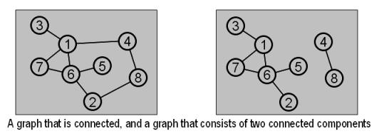
More formally, a connected component is a subgraph with the following two properties:
The length of a path or walk is the number of edges that it uses, counting multiple edges multiple times. In the graph below, (5, 2, 1) is a path of length 2 and (1, 2, 5, 1, 2, 3) is a walk of length 5.
The distance between two vertices x and y is written d(x,y) and defined as the length of the shortest path from x to y. If there is no path from x to y (i.e., if x and y are in different connected components), then d(x,y) is infinity.
The diameter of a graph G is the maximum distance between any two vertices in G. If G is not connected, then the diameter of G is infinity.
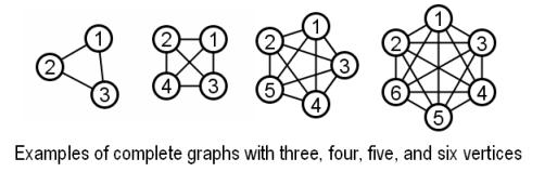
In a complete graph, every pair of vertices is joined by an edge.
Given a graph, a clique is a subset of vertices such that every pair of vertices in the subset is joined by an edge. The size of a clique is the number of vertices it contains. The red nodes {6,8,12} below are a clique of size three:
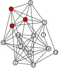
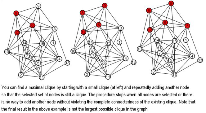
It is an interesting and very hard problem to find the largest clique in a graph-- known as the maximum clique problem. Can you find the largest clique in the graph above? Below is an example of an easier version of this problem.
The opposite of a clique is an independent set. An independent set is a subset of vertices such that for every two vertices in the subset, there is no edge connecting the two. The size of an independent set is the number of vertices it contains. 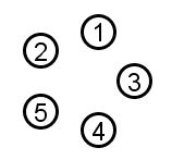
The vertices of any edgeless graph make an independent set, rather trivially:
Given an arbitrary graph (with edges), it is an interesting and hard problem to find the largest independent set in the graph. This is known as the maximum independent set problem. The blue nodes below are a maximum independent set:

It is often useful to consider only part of a graph. Induced subgraphs are one particularly convenient way to define a specific sub-part of a larger graph.
 Graph G = (V,E) |
 Subgraph induced by subset of nodes {1,2,3,4} |
Given a graph G=(V,E), an induced subgraph is defined by a subset of vertices S ⊆V. Then the nodes of the subgraph induced by S are simply the nodes in S, and the edges of the subgraph induced by S are all edges with both endpoints in S.
The upper graph pictured at right shows G=(V,E) with V={x: x is an integer from 1 to 8} and edges as drawn.
The lower picture shows the subgraph induced by the subset of nodes S={1, 2, 3, 4}. Notice that this induced subgraph consists of two connected components, even though the graph as a whole is a single connected component.
Another Example: In lecture we have discussed the Facebook friends network. We can write this as a graph using implicit notation as follows: G = (V,E), where V = {x: x is a person on Facebook} and E = {{x,y}: x V and y V and (x and y are friends on Facebook)}. The Facebook friends network is enormous, and so graph G is impossible to draw by hand; however, we can choose a small subset S of nodes in V and draw the graph induced by that subset S. This is exactly what the Touchgraph Facebook browser does: It lets you choose set S to be some number of your "Top Friends" on Facebook, possibly with the addition of yourself. Given this set S, Touchgraph displays a subgraph of the entire Facebook friends network: specifically, the subgraph induced by your chosen number of "Top Friends" (possibly with the addition of yourself).
Below is the subgraph of the Facebook friends network induced by the subset S={Patti, Jenny, Bill, Deborah}. This set S is exactly Bruce Hoppe's "Top 4 Friends" (which does not include Bruce Hoppe). The edges are hard to see but they are {{Patti, Jenny}, {Jenny, Bill}, {Bill, Patti}, {Bill, Deborah}}. There are no edges joining Deborah and Patti, or Deborah and Jenny, because these people are not Facebook friends.

The clustering coefficient C(x) for a node x measures the extent to which neighbors of x are also neighbors of each other. We can define the clustering coefficiently very neatly by combining these three concepts:
Note that we have defined all three of these concepts earlier. Now we combine them to define the clustering coefficient of a node x as follows:
The clustering coefficient of a node x is C(x) = the density of the subgraph induced by the neighborhood of x. |
Let's consider a few examples based on the following graph:

The clustering coefficient of node 2:
Step 1: The neighborhood of node 2 is N(2) = {17, 4, 10, 19, 6, 18, 15}.png)
Step 2: The subgraph induced by N(2) is indicated by the dark nodes and edges drawn at right. Node 2 is not an element of its own neighborhood, and the light gray edges are not part of the subgraph; those light gray elements are drawn just to provide context for the actual subgraph induced by N(2).
Step 3: Calculate the density of the induced subgraph using the usual formula, where our node set N(2) has 7 nodes and our edge set has 7 edges.
The maximum possible number of edges in the subgraph is
|N(2)|*(|N(2)|-1)/2 = 7 * 6/2 = 21
And the density of this subgraph is
= (actual # edges with both endpoints in N(2)) / (max possible # edges)
= 7/21 = 1/3
Thus the clustering coefficient of node 2 is 1/3.
The clustering coefficient of node 8:
Step 1: The neighborhood of node 8 is N(8) = {18, 6, 20, 12, 9, 15} .png)
Step 2: The induced subgraph is drawn at right (again the subgraph is indicated by dark nodes and edges and light gray elements are shown just for context)
Step 3: Calculate the density of the induced subgraph.
Number of nodes = 6
Number of edges = 5
Density = 5/(6*5/2) = 5/15 = 1/3
In this example, we again end up with a clustering coefficient of 1/3
The clustering coefficient of node 13:
Step 1: The neighborhood of node 13 is N(13) = {11, 14, 5, 9, 12, 16} .png)
Step 2: The induced subgraph is drawn at right (again the subgraph is indicated by dark nodes and edges and light gray elements are shown just for context)
Step 3: Calculate the density of the induced subgraph.
Number of nodes = 6
Number of edges = 8
Density = 8/(6*5/2) = 8/15
So the clustering coefficient of node 13 is 8/15.
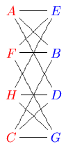
A more intuitive way to think of a bipartite graph is as a graph whose nodes can each be colored red or blue such that there are no red-red edges and no blue-blue edges. The following graph, for example, is bipartite and so can be colored red and blue without creating red-red edges or blue-blue edges:
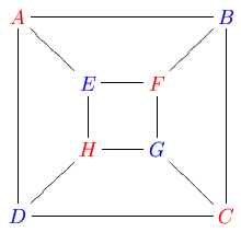
Another way to think of a bipartite graph is by drawing the red nodes on one side of the picture and the blue nodes on the other side of the picture:
 saying the same thing. For example, the following graph is non-bipartite:
One application of bipartite networks is the organization of user-created tags, such as the tags in del.icio.us. Together with the website URLs they are associated with, these tags form a bipartite network. For example, the yellow nodes below left are tags on del.icio.us, and the orange nodes below right are some of the URLs associated with these tags:
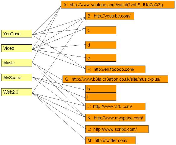
Even a machine that doesn't understand the tag-words themselves can analyze how the tag-words relate to each other based on how others associate those tags with website URLs.
The simplest indicator of tag relatedness is the group interlock network, which is explained in Six Degrees. Unfortunately, the group interlock network is too crude for many purposes, because it provides only a yes/no indicator and does not indicate relative amount of relatedness.
A more useful measurement of tag (or node) relatedness is based on comparing network neighborhoods. Two nodes (or tags) with similar neighborhoods are closely related to each other; two nodes with completely different neighborhoods are not at all related, and there are many possible shades of grey in between.
In the example above, the neighborhoods of YouTube and Video have many nodes in common and so they are closely related. By contrast, the neighborhoods of MySpace and Video have no nodes in common and so they are not at all related (in the example--probably different case than real life).
We formalize this notion by defining the structural equivalence of two nodes x and y as
SE(x,y) = |N(x) ∩ N(y)| / |N(x) ∪ N(y)|
This equals 1 when two nodes have identical neighborhoods (i.e., two tags have identical website associations) and 0 when two nodes have mutually exclusive neighborhoods (i.e., two tags have not a single common website associated with them).
Examples:
The structural equivalence of YouTube and Video is
|N(YouTube) ∩ N(Video)| / |N(YouTube) ∪ N(Video)|
= |{A, B, C, F} ∩ {A, B, C, D, E, F}| / |{A, B, C, F} ∪ {A, B, C, D, E, F}|
= |{A, B, C, F}| / |{A, B, C, D, E, F}|
= 4 / 6
= 2/3
The structural equivalence of MySpace and Video is
|N(MySpace) ∩ N(Video)| / |N(MySpace) ∪ N(Video)|
=|{H, I, K} ∩ {A, B, C, D, E, F}| / |{H, I, K} ∪ {A, B, C, D, E, F}|
=|{ }| / |{A, B,C, D, E, F, H, I, K}|
= 0 / 9
= 0
A tree is a graph in which any two vertices are connected by exactly one path.
Here are three different trees made from the same set of nodes:

In computer science, we often use trees for hierarchical organization of data, in which case we use rooted trees.

In the above tree, node 3 is specially designated as the root of the tree. Every other node in the tree is implicitly ranked by its distance from the root.
For any edge in a rooted tree, one end of the edge must be closer to the root than the other. We call the node closer to the root the parent of the other node, and we call the node farther from the root a child of its parent node. For example, nodes 9 and 4 are children of node 3. Similarly, nodes 10, 6, and 5 are all children of node 4. (And node 2 is the only child of node 9.) Any node in a rooted tree may have any number of children (including zero). A node with no children is called a leaf (examples leaf nodes are 1, 10, 7, and 5). Every node except the root node must have exactly one parent. For example, the parent of node 7 is node 6. Note that the above rooted tree is undirected, but each edge in the rooted tree has an implicit direction based on the parent-child relationship represented by that edge.
Any node of a tree can be a valid root of that tree. For example, if we decided that node 6 was actually the central anchor of the above network, we could re-root the exact same tree at 6 instead of 3:

Check and see that the two graphs above have exactly the same sets of nodes and edges. What happens to parent-child relationships when a tree is re-rooted?
In terms of its graph theoretic properties, a rooted tree is equivalent to the traditional hierarchical organizational chart:

The Division Officer at the top of the above hierarchy would probably argue that changing the root of the corresponding tree is a bad idea. However, if we are using trees to connect computers or concepts rather than people, we are less likely to encounter resistance when considering different alternatives for designating the root of a tree.

Mathematical InductionWhen you write a computer program, how do you know it will work? A mathematical proof is a rigorous explanation of such a claim. (Example claim: "MapQuest finds the shortest path between any two addresses in the United States.") A proof starts with statements that are accepted as true (called axioms) and uses formal logical arguments to show that the desired claim is a necessary consequence of the accepted statements.Mathematical induction (or simply induction) is one of the most important proof techniques in all of computer science. Induction is a systematic way of building from small example cases of a claim to show that the claim is true in general for all possible examples. Every proof by induction has two parts:
Suppose we want to prove that the maximum possible number of edges in an undirected graph with n nodes is n*(n-1)/2. Let's prove this by induction:

The maximum number of edges incident to node i+1 is simply i (which would happen if node i+1 is adjacent to every other node in the graph). Adding the above two terms gives us the maximum number of edges in a graph with n=i+1 nodes equal to
Voila! Check for yourself that we have completed both the base case and the inductive step. We now have a complete proof by induction that the maximum number of edges in a graph with n nodes is n*(n-1)/2. |

# edges in blue sub-tree = # edges in green sub-tree = # edges in yellow sub-tree = |
|Vblue| - 1 |Vgreen| - 1 |Vyellow| - 1 |
# edges in all sub-trees = |
i - 3 |
|E| = |
i - 3 + 3 = i |

We will apply Kruskal's algorithm to the graph above. Recall that set F initially includes every edge. Set T is initially empty. As we add edges to T in the example below, we color those edges green.
|
This is our original graph. The numbers near the arcs indicate their weight. None of the arcs are highlighted. |
|
{A,D} and {C,E} are the shortest arcs, with length 5, and {A,D} has been arbitrarily chosen, so it is highlighted. |
|
However, {C,E} is now the shortest arc that does not form a cycle, with length 5, so it is highlighted as the second arc. |
|
The next arc, {D,F} with length 6, is highlighted using much the same method. |
|
The next-shortest arcs are {A,B} and {B,E}, both with length 7. {A,B} is chosen arbitrarily, and is highlighted. The arc {B,D} has been highlighted in red, because it would form a cycle (A,B,D,A) if it were chosen. |
|
The process continutes to highlight the next-smallest arc, {B,E} with length 7. Many more arcs are highlighted in red at this stage:
|
|
Finally, the process finishes with the arc {E,G} of length 9, and the minimum spanning tree is found. |
The core network mathematical concept in Google rankings is the notion of centrality. This is an intuitive notion that is surprisingly hard to pin down mathematically. For example, which node is the most central in the following graph?
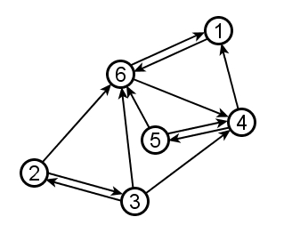
There is no one right answer to the question, because the question is too vague. There are many different ways to define centrality more precisely. Here are three important ones, all of which rely critically on the direction of links (something we have been glossing over until now):
The PageRank formula is described and illustrated with examples and an interactive PageRank calculator at http://www.webworkshop.net/pagerank.html.
WebWorkshop writes the PageRank formula in a manner that is compact but subtle. We restate the formula here and then introduce an easier, simplified forumulation. We begin by defining a damping factor d to be a fixed coefficient at least 0 but no more than 1. (A typical value is d=0.85.) Then for any graph, we define the PageRank of each of its nodes as follows:
For any node x, let
Then PageRank(x) =
|
Computing PageRank from the above definition presents both major and minor difficulties:
Here we present Compounded Indegree Centrality as a simple way to estimate PageRank. It is equivalent to the PageRank formula referenced above with damping coefficient d=1 and with no dividing by node outdegrees. Compounded indegree centrality will proceed iteratively, by first calculating InDegree1, then InDegree2 based on InDegree1, and so forth.
Using the same 6-node graph as above, we start by defining the InNeighborhood of a node x to be all nodes that have directed edges into x. Then the InDegree1 of a node is simply the cardinality of its InNeighborhood--just another name for indegree.
| Node |
InNeighborhood |
InDegree1 |
| 1 |
{4,6} |
2 |
| 2 |
{3} |
1 |
| 3 |
{2} |
1 |
| 4 |
{3,5,6} |
3 |
| 5 |
{4} |
1 |
| 6 |
{1,2,3,5} |
4 |
InDegree1 is a very local measure of node centrality. We can measure a slightly more system-wide sense of node centrality by defining InDegree2 as follows:
For any node x, InDegree2 of x is the sum of the InDegree1's of all nodes in the InNeighborhood of x.
| Node |
InNeighborhood |
InDegree1 |
InDegree2 |
| 1 |
{4,6} |
2 |
7 = 3+4 |
| 2 |
{3} |
1 |
1 = 1 |
| 3 |
{2} |
1 |
1 = 1 |
| 4 |
{3,5,6} |
3 |
6 = 1+1+4 |
| 5 |
{4} |
1 |
3 = 3 |
| 6 |
{1,2,3,5} |
4 |
5 = 2+1+1+1 |
We can then repeat the above process to calculate InDegree3 based on InDegree2, then InDegree4 based on InDegree3, etc. Below is a table of five successive calculations of InDegree, based on the same graph as above:
| Node |
InNeighborhood |
InDegree1 |
InDegree2 |
InDegree3 |
InDegree4 |
InDegree5 |
| 1 |
{4,6} |
2 |
7 |
11 |
21 |
38 |
| 2 |
{3} |
1 |
1 |
1 |
1 |
1 |
| 3 |
{2} |
1 |
1 |
1 |
1 |
1 |
| 4 |
{3,5,6} |
3 |
6 |
9 |
19 |
29 |
| 5 |
{4} |
1 |
3 |
6 |
9 |
19 |
| 6 |
{1,2,3,5} |
4 |
5 |
12 |
19 |
32 |
Below we redraw the same table, highlighting exactly how the row for node 4 is calculated. Because the InNeighborhood of node 4 is {3,5,6}, in each iteration the compounded indegree of node 4 takes the values of nodes 3, 5, and 6 from the previous column.
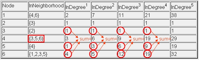
Notice also that the rankings of relative node centrality change from column to column in the above table. Sometimes node 6 is most central; sometimes node 1 is most central. After "enough" iterations, the rank order of relative node centrality will stabilize.


